KAME
KAME: AI-Assisted Automation Program for Physical Property Measurements




KAME is an open-source, multi-threaded program for automated physical property measurements, developed at Kitagawa Laboratory, ISSP, University of Tokyo. It is particularly suited to NMR and ODMR experiments, and supports AI-assisted measurement orchestration across compatible instruments.
License: GPL v2 or later (prior to 8.0: LGPL v2 or later)
Authors: Kentaro Kitagawa, Shota Suetsugu
Platforms: macOS, Windows (64-bit), Linux (x86-64, supported from 8.5 — see INSTALL.linux)
Manual: 日本語 · English
Paper: K. Kitagawa, Formally Verified Lock-Free Software Transactional Memory for Scientific Measurement, arXiv:2608.12024 (2026)
Features
- Transactional, lock-free node/data model (Software Transactional Memory) —
spun out as the dual-licensed reusable libraries
kamestm/(STM core) andkamepoolalloc/(four-tier pool allocator) — see Reusable subsystems - Python (+Jupyter notebook) and Ruby scripting — nearly full control from scripts
- AI-assisted experiment automation via MCP — Claude Code, Codex, Antigravity, Claude Desktop, LM Studio / Bionic and any other MCP client (local models included, through Pydantic AI) can read instruments, control parameters, and run measurement sequences through natural language, with the instrument-safety rules delivered by the server itself
- OpenGL-based 2-D / 1-D graph display; arbitrary scalar combinations (T, V, …)
- Real-time NMR relaxation fitting (T1, T2, Tst.e.), Inverse Laplace Transform
- Fourier step-sum spectrum measurement with field / frequency sweeping
- Complete data logging with post-measurement re-analysis
- Save / restore full measurement config to
.kamfiles - Provenance journal: settings and every change to them in
.kamj, raw records in.kamb, either file replayable (9.0) - Modular driver plug-in architecture; Python drivers redefinable at runtime
- Calibration curves (cspline, Chebyshev, polynomial) for resistance thermometers and generic sensors; calibrated entries feed into graphs, charts, and data recording like any native scalar
Released versions/Binaries
Source: kame-8.6.1.zip (3.7MB, Aug. 2026). All other source archives. Windows 64-bit binaries: 8.6.1 (21.8MB) · 8.6 (21.8MB) · 8.5 (20.4MB) · 8.4. At least Qt is additionally needed, follow instructions below to install. Builds before 8.6.1 carry the double-allocation defect described under What’s New in 8.6.1 on Windows and Linux. 9.0 alpha2 — the measurement journal, below: source (3.8MB) · Windows 64-bit. A pre-release; 8.6.1 remains the current stable version.
Supported instruments
| Category | Models |
|---|---|
| Oscilloscopes (DSO) | Tektronix TDS, Lecroy/Teledyne/Iwatsu, Thamway PROT3 streaming DSO, Thamway DV14U25 A/D board, NI-DAQmx as DSO, Digilent WaveForms AIN |
| Signal generators | Kenwood SG7130/7200, HP/Agilent 8643/8644/8648/8664/8665, Keysight/Agilent E44xB SCPI, Rohde-Schwarz SML01/02/03/SMV03, DSTech DPL-3.2XGF, LibreVNA SG SCPI |
| Function / pulse generators | NF WAVE-FACTORY, LXI 3390 arbitrary function generator |
| Network analysers | HP/Agilent 8711/8712/8713/8714, Agilent E5061/E5062, Copper Mountain TR1300/1504/4530, DG8SAQ VNWA3E, LibreVNA SCPI, Thamway T300-1049A impedance analyser |
| Lock-in amplifiers / bridges | Stanford SR830, NF LI5640, Signal Recovery 7265, LakeShore M81-SSM, Agilent/HP 4284A LCR meter, Andeen-Hagerling 2500A capacitance bridge |
| DC sources | Yokogawa 7651, Advantest TR6142/R6142/R6144, MICROTASK/Leiden triple current source, Optotune ICC4C-2000 |
| Multimeters / picoammeters | Keithley 2000/2001, 2182 nanovolt meter, 2700+7700, 6482 picoammeter; Agilent 34420A, 3458A, 3478A; Sanwa PC500/5000 |
| Temperature controllers | Cryocon M32/M62, LakeShore 218/340/350/370/372 (1ch, 8ch, 16ch scanner), Picowatt AVS-47, Oxford ITC-503, Neocera LTC-21, Scientific Instruments 9302/9304/9308, LinearResearch LR-700, OMRON E5*C Modbus |
| Magnet power supplies | Oxford PS-120, Oxford IPS-120, Cryogenic SMS10/30/120C |
| NMR pulsers | Thamway N210-1026 PG32U40 (USB), PG027QAM (USB), N210-1026S/T (GPIB/TCP); NI-DAQ analog+digital output, digital output only, M+S Series; handmade H8, handmade SH2 |
| NMR / RF measurement | Thamway PROT NMR (USB/TCP), NMR FID/echo analyser, T1/T2 relaxation, field-swept spectrum, frequency-swept spectrum, NMR built-in network analyser, NMR LC autotuner |
| Cameras / imaging | IEEE 1394 IIDC, Euresys eGrabber (CoaXPress), Euresys Grablink (CameraLink), Hamamatsu via Grablink, JAI via Grablink, OceanOptics/Insight USB/HR2000+/4000 spectrometer |
| Laser modules | Coherent Stingray, Newport/ILX LDX-3200, Newport/ILX LDC-3700(C) |
| ODMR | Frequency-swept spectrum, FM peak tracker, 2-D image analysis, filter wheel (STM-driven) |
| Motors / positioners | OrientalMotor FLEX CRK, CVD2B, CVD5B, FLEX AR/DG2, EMP401; SigmaOptics PAMC-104 piezo-assisted; Micro CAM z/x/φ; Two-axis rotator |
| Flow controllers | Fujikin FCST1000 series |
| Level meters | Oxford ILM helium level meter, Cryomagnetics LM-500 |
| Vacuum gauges | Pfeiffer TPG361/362 |
| Pump controllers | Pfeiffer TC110 turbopump controller |
| Counters | Mutoh Digital Counter NPS |
| Quantum Design PPMS | PPMS low-level interface |
| NI DAQmx | Pulser (AO+DO, DO-only, M+S Series), DSO |
| Resistance measurement | Four-terminal with polarity switching; Python-based 4-terminal (simple and multi-current variants) |
| Monte Carlo simulation | Monte Carlo driver |
What’s New in 9.0 (alpha)
- KAME records what it was set to and what it did, without being asked. A
run is one name and two files. The
.kamjholds the settings the run started with, and every change made afterwards, yours and the instruments’. The.kambholds the raw records behind those readings. You choose whether the second file is written at all: settings alone cost about 11 MB/hour at 144 readings a second, settings plus records about 10 GB/hour. Both files are gzip, and.kamjis JSON Lines inside, sozgrepandzdiffread one with no special tool. Numbers are stored twice, as the text you would read and as the exact eight bytes they were. - The session is recorded even when you are not recording a run. It goes to a directory of its own and stays at a few tens of KB. Everything you did is kept in full; an instrument’s readings are kept only once they settle. A session you forgot to save now has something to show.
- Replay, in the Journal Reader. Open either file and the other is found.
Open the
.kamjand the settings of each moment come back as playback reaches them. Open the.kamband the same records are re-analysed with the settings you have now, which is what you want after changing one parameter. Drivers named in the journal are created if this KAME does not have them. Only what a person set is restored, never into a running driver, and KAME reports how much it held back. - The toolboxes and the main window get out of the way by themselves. A toolbox at a screen edge shrinks to its tab column, and grows back when the pointer touches it. The main window keeps its top edge and rests at half height, so the menu bar and the pane tabs never move. Hovering a tab picks that pane, which makes a resting toolbox a menu of its panes. Click the front tab to pin a window open. Both are switches in the View menu.
- Smaller UI changes. The New Driver dialog has a live search box. A driver you create opens its own window, and one with an interface brings up the Interface pane. The pane tabs are flat and move faster. An interface that appears is selected and scrolled to. On macOS, choosing KAME in the Dock brings the main window forward.
What’s New in 8.6.1
- A block of memory could be handed out twice — Windows and Linux. Frees arriving from a thread that had already finished its own allocator teardown went into an object that no longer existed, and a slot went back to the pool after its owner had already reissued it, so two live users held the same memory. It surfaced far from its cause and never the same way twice: garbage inside a value still being referenced, a node that reported the wrong identity, or the transaction watchdog firing on a stall that was not one. macOS was never affected — the guard that was supposed to prevent this compiled to a constant false everywhere else. 8.5 and 8.6 carry the defect on Windows and Linux; update.
- The MCP pre-check no longer cries wolf. On Windows, KAME could announce
that no Python with
mcpandjupyter_clientwas found — and then start the server anyway, on the next line. The startup pre-check probed candidates with KAME’s ownPYTHONHOMEstill set, which underkame-msyspython.batpoints a real CPython at MSYS2’s standard library and kills it on_socket; it now strips that environment, as the other probe already did. The same fix cures the Pydantic AI interpreter search. - The test suites build under MSVC, not only clang/MinGW, and every test that builds there passes.
What’s New in 8.6
- Windows: MCP works — and the release zip now actually contains it. Nothing deployed
scriptfile.fileson Windows (they sat inDISTFILES, which copies nothing), andmkzip.batpackaged the build tree’sresources\wholesale, so whetherkame_mcp_server.pyreached a release depended on whether someone had once hand-copied it there. The 8.4 and 8.5 Windows binaries could therefore be missing it, and the resultingcan't open file …\Resources\kame_mcp_server.pygave no hint that the fix was to fetch the file from the source archive. Both a build and a release now runtools/deploy_scripts.bat, so they get an identical, complete set. Three further faults each hid the next:pip install mcpnow serves 2.x without themcp.server.fastmcpthe server imports, the MSYS2 launcher’sPYTHONHOMEwas inherited by a real CPython that cannot load mingw extensions, andFastMCP.run(host=…)is aTypeErrorin mcp 1.x. - Permanent client registration. One Script-pane action registers KAME with Codex, Antigravity CLI (
agy) and Claude Desktop, each through the mechanism that client provides, and reports every change before it writes. LM Studio / Bionic need nothing — a project opened on the notebook workspace reads the.mcp.jsonKAME already writes there. - The model stays yours. The Pydantic AI links hand KAME’s agent to your own
clai(clai -a kame_pydantic_ai:agent), so provider, keys and default come from the setup you already have and KAME never asks which model to use. - Agent plugin: the MCP server and a
kame-measurementskill as one directory, both a Claude Code plugin and an Agent Plugins 1.0.0 one. - Usage records: one JSONL line per MCP tool call and per model request — counts and timings only, never prompt or response text.
- Windows: the Claude and Codex desktop links open the apps, which ship as MSIX and are reachable only by AppUserModelID.
- macOS: idle CPU back to a few percent — the main loop never asked to wait, so it could not sleep.
- The Jupyter server exits with KAME instead of orphaning itself; a second click reopens the running one.
- MCP async jobs can read their own thread context, and tracebacks arrive without IPython’s colour escapes.
What’s New in 8.5
- Linux is a supported platform — Qt 6 / qmake, verified on Ubuntu 26.04 including
PREEMPT_RT. Two paths have real hardware behind them: the Thamway FX2/FX3 USB path, whose first Linux run found and fixed four crashes, and the usermode NI USB-GPIB driver. SeeINSTALL.linux. - Crash audit with automated checkers —
tools/audit/run_audits.shmechanically enforces the driver-authoring rules (node-name collisions, side effects initerate_commitclosures, pybind GIL discipline, UI-touching listeners, non-const Payload pointees), as a pre-commit hook and in CI. - Pulser correctness — overlapping RF pulses are refused rather than played, two operator-precedence bugs that left the amplifier gate open are fixed, and the
ASWSetupclamp that recursed on itself is gone. - One-click Codex launch — Codex and codex-fugu join Claude Code in the Script pane, each started already pointed at this KAME’s MCP server.
What’s New in 8.0
- MCP server for AI-assisted experiment automation — built-in Model Context Protocol server lets AI assistants (Claude Code, Claude Desktop, etc.) execute Python code in the running KAME process, read instrument values, and control measurements through natural language. Matplotlib plots are returned inline. Long-running experiments (sweeps, scans) run asynchronously.
- Calibrated scalar entries —
XCalibratedEntryapplies a calibration curve to any scalar entry; the result appears in graphs, charts, and data recording like a native scalar. - Usermode NI USB-GPIB on Apple Silicon — the embedded userspace linux-gpib port now works reliably on macOS ARM64 without any kernel module.
- Window cascade placement — instrument windows are automatically arranged on show.
- Comprehensive bug audit — 20 bug fixes across 12 source files (GIL safety, buffer bounds, null-pointer guards, logic errors).
- Arbitrary masks for 2D math tools — Rectangle, Ellipse, or a binary mask set from Python; highlights render as GPU textures.
- Math tool API cleanup — ROI endpoints renamed
Begin/EndtoFirst/Last(inclusive); old.kamfiles still load.
Architecture
Reusable subsystems
Two pieces of KAME’s foundation are maintained as stand-alone dual-licensed libraries (Apache 2.0 OR GPL-2.0-or-later) within this monorepo, intended to be carved out as their own subtrees for downstream embedding:
kamestm/— Lock-free software transactional memory. The snapshot / transaction core (Node<XN>,Snapshot<XN>,Transaction<XN>; plus theatomic_shared_ptr<T>engine, homed inkamepoolalloc/) extracted as a header-only library plus three small.cpp(threadlocal/xthread/xtime). TLA+ specs for the protocol; GenMC RC11-checked C translations. Builds on macOS clang / Linux gcc/clang (64+32-bit) / Windows MinGW + MSVC, and the registered standalone test suite passes on each (the exact test count is platform-dependent). Seekamestm/README.md.kamepoolalloc/— Four-tier lock-free pool allocator. 1 B to multi-GiB span (buckets / dedicated chunks / largemmap/ huge), per-thread DLL + cross-thread coalescing, two-level recycle cache, TLA+ / GenMC verified, drop-innew/deletereplacement. Coexists with foreign allocators on every OS via the native interposition: ELF strong symbols on Linux, Mach-O__DATA,__interposeon macOS, free-family IAT redirect on Windows (§31). Builds on the same four toolchains; MSVC live pool is default-on (opt OUT withKAME_DISABLE_POOL_MSVC). Included in mimalloc-bench askp, so it can be measured against the usual field with the suite’s own harness. Seekamepoolalloc/README.mdand the INVARIANTS / SUBSYSTEMS navigation map.
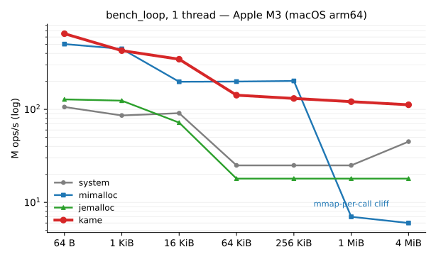
kamepoolalloc vs system / mimalloc / jemalloc — single-thread malloc/free
sweep on Apple M3. No size cliff; full benchmarks
(x86-64 bare metal, 128-core scaling, mimalloc-bench suite).
The rest of this Architecture section describes how KAME itself uses these
pieces — instrument drivers, Python integration, .kam serialization, and
how the STM machinery from kamestm/ is wired into the node tree.
Driver / Plug-in Architecture
Instrument drivers are shared libraries under modules/ loaded at runtime via ltdl.
Each driver subclasses XDriver (kame/driver/driver.h), which carries a timestamped
Payload (time() = phenomenon time, timeAwared() = acquisition start time) and emits
onRecord / onVisualization signals.
Hardware communication is abstracted in modules/charinterface/ (serial, TCP, GPIB, USB).
Drivers can also be subclassed in Python via XPythonDriver (kame/driver/pythondriver.h).
Scalar values extracted from driver records are represented as XScalarEntry objects
(kame/analyzer/). A derived XCalibratedEntry applies any registered calibration curve
to an existing entry, and the result appears in graphs, charts, and data recording
exactly like a native scalar. Calibration curves (kame/thermometer/) include cubic
spline (XApproxThermometer, XGenericCalibration), Chebyshev polynomial (XLakeShore),
and polynomial (XScientificInstruments) types. XGenericCalibration supports
user-configured labels and units, making it applicable to any sensor, not just thermometers.
Usermode NI USB-GPIB
modules/charinterface/usermode-linux-gpib/ contains a userspace port of the NI USB-GPIB
kernel driver from linux-gpib 4.3.6. The upstream ni_usb_gpib.c is minimally patched
(Linux-only headers guarded with #ifdef __KERNEL__); a compatibility header
(osx_compat.h / win_compat.h) replaces every Linux kernel API — kmalloc, spinlocks,
wait queues, USB URBs — with POSIX/libusb or Win32 equivalents.
The result is a standalone executable that speaks to NI USB-B, USB-HS, USB-HS+, KUSB-488A, and MC USB-488 adapters on macOS, Linux, and Windows without installing a kernel module or any proprietary driver. On macOS this is the only viable path for USB-GPIB on Apple Silicon.
Python Integration
This section was drafted with AI assistance (Anthropic Claude) and technically reviewed and verified by the maintainers.
Python access is provided via pybind11. The embedded interpreter runs in its own OS thread; the Qt main thread and the Python thread communicate through the Talker/Listener signal mechanism.
Accessing the node tree from Python:
root = Root()                      # root of the instrument node tree

# Read a value (Snapshot)
shot = Snapshot(root)
print(shot[root])                  # payload of the root node

# Navigate children
tempcontrol = root["tempcontrol"]  # by name
print(float(tempcontrol["temp"]))  # XDoubleNode coerces to float

# Write a value (Transaction)
for tr in Transaction(tempcontrol["setpoint"]):
    tr[tempcontrol["setpoint"]] = 4.2   # retry loop, just like C++
Writing instrument drivers in Python:
Any C++ driver base class can be subclassed in Python via XPythonDriver<T>.
The subclass is registered at runtime with exportClass() and instantiated by the
framework exactly like a compiled driver. This enables rapid prototyping of new
instrument interfaces without recompiling KAME.
class MyDriver(kame.XPythonCharDeviceDriverWithThread):
    def analyzeRaw(self, reader, payload):
        payload.local()["value"] = float(reader.pop_string())
    def visualize(self, shot):
        ...
MyDriver.exportClass("MyDriver", MyDriver, "My Instrument")
The driver’s Payload.local() dict is deep-copied per transaction, giving Python
state the same snapshot-isolation semantics as C++ Payload fields.
Jupyter notebook support:
KAME optionally embeds an IPython kernel. When IPython is available, a Jupyter client
can connect to the running process for interactive exploration and live plotting
alongside the native KAME UI. The kernel integrates with the asyncio event loop via
a custom ipykernel integration (loop_kamepysupport).
AI-assisted experiment automation (MCP):
KAME includes an MCP (Model Context Protocol) server
that lets an AI assistant execute Python code directly in the running KAME interpreter.
The MCP server connects to the embedded IPython kernel, giving the AI full access to
Root(), Snapshot(), Transaction(), and all loaded drivers — the same environment
available in Jupyter notebooks. Any MCP client works: Claude Code, Codex, Antigravity, Claude Desktop, LM Studio / Bionic, and a bundled
Pydantic AI client that reaches any provider:model, local models included.
This enables scenarios like:
- Conversational experiment control (“sweep temperature from 100 K to 300 K and record resistance”)
- Automated data collection with adaptive logic
- Real-time monitoring and analysis
See MCP setup below for configuration.
Threading notes:
- Long-running C++ calls release the GIL (
gil_scoped_release) so the Python thread does not block Qt. - Any Qt UI operation (loading
.uifiles, showing forms) must be dispatched to the main thread viakame.kame_mainthread(closure). - Payload garbage collection uses a deferred deque + mutex to avoid holding the
GIL during snapshot cleanup (GIL-enabled builds only); Python 3.13 free-threading
(
Py_GIL_DISABLED) is also supported.
Serialization (.kam files)
A .kam file is a Ruby script generated by XRubyWriter and re-executed on load.
Nodes marked runtime=true are written as comments and not restored.
XListNode children are recreated via createByTypename(); the typename must match
the key registered in XTypeHolder.
Software Transactional Memory (STM)
KAME’s core data model is a lock-free, snapshot-based STM
(kamestm/transaction.h — see Reusable subsystems).
All instrument data lives in a tree of Node<XN> objects; reads and writes are
expressed as snapshots and transactions rather than locks.
Node<XN>
 └─ Linkage  ──atomic_shared_ptr──▶  PacketWrapper
                                          └─ Packet
                                              ├─ Payload   (user data)
                                              └─ PacketList (child packets)
Reading — O(1) snapshot:
Snapshot<NodeA> shot(node);         // atomic load, no lock
double x = shot[node].m_x;
Writing — optimistic transaction with automatic retry:
node.iterate_commit([](Transaction<NodeA> &tr) {
    tr[node].m_x += 1;             // copy-on-write on first access
});                                 // retried automatically on conflict
How commits work:
Transactionsavesm_oldpacketat construction.operator[]clones the payload (copy-on-write) on first write, stamping it with a unique serial.commit()does a single CAS onLinkage; ifpacket != m_oldpacketa conflict is detected and the transaction retries.- Listeners receive deferred events only after a successful commit — no intermediate states are visible.
Lock-free atomic shared pointer
The O(1) snapshot reads and CAS-based commits above require a shared
pointer that is itself lock-free. atomic_shared_ptr (introduced in
January 2006 as part of the 2.0-beta3 rewrite) provides this — a custom
implementation of what C++20 calls std::atomic<shared_ptr>, built on
tagged-pointer CAS with a small local reference counter packed into the
pointer’s low bits. It lives in
kamepoolalloc/atomic_smart_ptr.h,
the single shared home for the lock-free primitives that BOTH the STM
and the pool allocator rely on.
Technique deep-dive (local + global refcount, intrusive
atomic_countable path, comparison against the libstdc++ / MSVC / libc++
std::atomic<shared_ptr> implementations) lives in
kamestm/README.md § Lock-free atomic shared pointer
— single source of truth, shared with the standalone kamestm library
release.
Multi-node consistency is achieved through a bundling protocol: a parent packet absorbs child packets via multi-phase CAS protocol, making the entire subtree consistent under a single atomic pointer. A m_missing flag marks packets with stale children, driving re-bundling on demand.
Collision negotiation: when concurrent transactions repeatedly collide,
the negotiate machinery (ScopedNegotiateLinkage::_negotiate()) lets the
single oldest transaction win — each contended linkage is tagged with the
tagger’s start-time stamp (oldest-wins), a starved Tx escalating to a
privileged Reserved tag; non-privileged contenders park until it commits,
so the oldest/highest-priority Tx makes progress ahead of the contenders parked
behind it. Model-checked livelock-free in TLA+ (exhaustively for the checked,
finite thread counts and tree shapes — not a proof for arbitrary deployment
sizes). Full details + the comparison
against other STMs (Haskell TVar / Clojure Ref / ScalaSTM, HTM TSX/RTM,
TinySTM / NOrec) live in kamestm/README.md — KAME’s
STM core is dual-licensed and maintained as a standalone library, with its
own design doc to avoid duplicating it here.
iterate_commit_while(lambda) lets the caller abort the retry loop (return false from the lambda to stop), enabling conditional transactions.
Caution: Taking a nested
Snapshotinside a transaction can trigger bundling, which may cause the transaction’s CAS to always fail. This is not a data corruption issue but a liveness issue — the transaction retries indefinitely. This occurs when theSnapshottarget is an ancestor of the transaction target, or when hard links exist (a child with two parents) and aSnapshoton one parent’s tree interferes with the other. Usetr[*node]instead of a nestedSnapshotin these situations.The hard-link case is now formally modelled in
kamestm/tests/tlaplus/BundleUnbundle_hardlink_*.tla(seven topology/pattern variants, incl. the conditional nested-sub-bundle gate-scope model); seekamestm/tests/VERIFICATION.md§5.
Why STM in a measurement framework
Laboratory software must acquire data on tight hardware timings while simultaneously updating a UI and running user scripts — all from different threads. Traditional mutex-based designs either serialize too aggressively (dropping samples) or require intricate lock ordering that is error-prone to extend. The STM approach offers three concrete benefits for this domain:
- Deadlock-free by design. No locks are held across hardware I/O or UI redraws, so a slow UI thread does not block a fast acquisition thread behind a lock.
- Consistent multi-instrument views. A
Snapshotof any subtree is always internally consistent — the UI always sees a coherent set of readings even when multiple drivers update simultaneously. - Safe scripting from Python/Ruby. Scripts read and write the node tree through the same transaction API as C++ code, so a user script cannot leave the node tree in a partially-updated state, whenever it runs.
For what makes KAME’s STM distinctive among STMs (tree-structured /
per-packet conflict granularity / bundling instead of read-write logs),
see the comparison tables in kamestm/README.md.
Formal verification (TLA+)
The STM protocol is formally specified and exhaustively model-checked with TLA+ / TLC for the documented finite thread counts and tree topologies. This is model checking of the protocol model, not a proof of the C++ implementation for arbitrary deployment sizes, compiler mappings, or real-time WCET:
- Layer 1 —
atomic_shared_ptr: tagged-pointer CAS protocol with local/global reference counting, drain release, andscoped_atomic_view(spec). Safety only — the bare primitive is intentionally not livelock-free. - Layer 2 — bundle/unbundle + commit: 2-/3-level subtree bundling with a livelock-free privileged-TID negotiate mechanism, static and dynamic (online insert/release) (2-level, 3-level, dynamic). Exhaustively model-checked safe + livelock-free without
CONSTRAINT(the LL-free design makes the state space naturally finite — no artificial bound); the largest single exhaustive run reaches ~641 M distinct states (3-level all-root, 15 h on the ISSP ohtaka supercomputer), over a billion across the LL-free configurations combined. (Raw state counts are spec-version-specific and shift as the spec evolves — see kamestm/tests/VERIFICATION.md §3–§4 for current-spec figures.) These are exhaustive results for the checked configurations (fixed thread counts and tree shapes), not an unbounded ∀-thread proof. - Hard-link topologies: multi-parent / one-child races that reproduce and fix a production abort via a Phase-4 reachability gate and a Phase-3 skip-Null fix (
kamestm/tests/tlaplus/BundleUnbundle_hardlink_*.tla).
Slide decks — start at the coverage overview (EN · JA), a hub linking every layer with a full coverage matrix. Individual decks (each with a Japanese counterpart under doc_ja/): Layer 1, Layer 2 base, Layer 2 LLfree, 3-level, dynamic, hard-link.
C11 translations of each layer are verified with GenMC under the RC11 memory model: TLA+-derived tests (kamestm/tests/tlaplus/test_*.c) and C++-derived protocol tests (kamestm/tests/cds_atomic_shared_ptr/). Full results: kamestm/tests/VERIFICATION.md.
Dependencies
| Library | Notes |
|---|---|
| Qt ≥ 5.7 or Qt 6 | Qt 6 needs uitools; the Qt5 compatibility module is no longer required |
| Ruby | scripting |
| pybind11 | Python scripting |
| GSL | |
| FFTW 3 | |
| Eigen 3 | |
| LAPACK / ATLAS / BLAS (optional) | |
| libtool-ltdl | runtime plug-in loading |
| zlib | |
| libusb | USB instrument interfaces |
| linux-gpib or NI 488.2 (optional) | GPIB interfaces |
| NI DAQmx (optional) | NI data-acquisition hardware |
A C++11-capable compiler is required (the build uses CONFIG += c++11 via qmake).
Optional: IPython / Jupyter notebook, linux-gpib or NI 488.2, NI DAQmx, libdc1394 (IIDC cameras, macOS/Linux), Euresys eGrabber SDK (frame grabbers).
Building
macOS
Open
kame.proin Qt Creator (use the genuine open-source Qt, not the MacPorts Qt).
Install dependencies via MacPorts:
sudo port install gsl fftw-3 libtool-ltdl libusb eigen3 pybind11
Optionally, for a universal (arm64 + x86_64) binary, build fftw-3 with:
sudo port install fftw-3 +universal +clang13 -gfortran
Additional notes:
- Add
/opt/local/binto PATH in the Qt Creator build-environment pane if needed. - In Qt Creator’s executable environment pane, deactivate “Add build library search path to DYLD_LIBRARY_PATH …”, otherwise KAME crashes on launch.
- If
ruby.his not found, reinstall Xcode command-line tools:xcode-select --install. - Qt 6: the Qt5 compatibility module is no longer needed — the last user of it was a dead
QTextCodecinclude, now removed. - NI 488.2 is not supported on Apple Silicon; use the built-in usermode NI USB-GPIB driver instead (no kernel module required).
Linux (x86-64, Qt 6 / GCC) — supported from 8.5
Build from source; there is no packaged Linux binary yet. Full notes, including the serial/GPIB smoke test and the remaining gaps, are in
INSTALL.linux.
Verified on Ubuntu 26.04, x86-64, including the PREEMPT_RT kernel the
realtime measurements below use.
sudo apt install -y \
    qt6-base-dev qt6-base-dev-tools qt6-tools-dev qt6-tools-dev-tools \
    libgl1-mesa-dev libglu1-mesa-dev \
    libgsl-dev libfftw3-dev libltdl-dev libeigen3-dev zlib1g-dev \
    libusb-1.0-0-dev ruby-dev python3-dev python3-pybind11
mkdir build && cd build
qmake6 ../kame.pro          # prints which Ruby and which Python it picked
make -j$(nproc)
./bin/kame                  # modules are found automatically; no --moduledir needed
Notes:
- The executable lands in
build/bin/kame, and the driver modules are grouped beside it underbin/{coremodules,coremodules2,modules}— which is whereQApplication::libraryPaths()looks, so the build tree runs as-is. - Ruby headers are mandatory (
script/xrubysupport.cppis compiled unconditionally).kame.proasks the interpreter viaRbConfig, so any packaged or rbenv/rvm Ruby works and its libdir is recorded as a RUNPATH. - pybind11 is optional but strongly recommended: without it there is no
Python scripting, no Jupyter/IPython console, no MCP server, and
.kamfiles fall back to the legacy Ruby loader.python3 -m pybind11 --includesmust succeed for the interpreter qmake selects. - Jupyter is a separate runtime dependency and must be installed into the
interpreter KAME embeds:
python3 -m pip install ipykernel ipython jupyter nest_asyncio numpy. - Installing:
qmake6 ../kame.pro PREFIX=/usr/local && make && sudo make installdeploys the binary, the modules to$PREFIX/lib/kame/, the scripts, manual and translations to$PREFIX/share/kame/, a.desktopentry, hicolor icons, and udev rules for the libusb instruments (kame/70-kame.rules). - GPIB: with linux-gpib headers present,
HAVE_LINUX_GPIBselects the native kernel-driver path; without them,Device = GPIBfalls back to the bundled usermode NI USB-GPIB driver (libusb, no kernel module).PrologixGPIBUSBis available either way. - Vendor SDKs (NI-DAQmx, Digilent WaveForms, Euresys eGrabber) are probed and enable their drivers when installed; when absent, those modules build but register nothing.
Windows (x86-64, MSYS2 / MinGW)
Requires Qt ≥ 6.10 with the llvm-mingw64 toolchain. Open
kame.proin Qt Creator.
Install dependencies via MSYS2:
pacman -S make \
    mingw-w64-x86_64-zlib \
    mingw-w64-x86_64-fftw \
    mingw-w64-x86_64-gsl \
    mingw-w64-x86_64-eigen3 \
    mingw-w64-x86_64-pybind11 \
    mingw-w64-x86_64-libusb \
    mingw-w64-x86_64-python-numpy \
    mingw-w64-x86_64-ruby
For the in-process Jupyter kernel and the notebook server (the
kame-msyspython.bat route below), add the notebook stack — MSYS2’s Python is
EXTERNALLY-MANAGED and ships no pip module, so these must come from
pacman, not pip:
pacman -S mingw-w64-x86_64-python-ipykernel \
    mingw-w64-x86_64-python-ipython \
    mingw-w64-x86_64-python-jupyter_notebook \
    mingw-w64-x86_64-python-pyzmq \
    mingw-w64-x86_64-python-matplotlib
python-jupyter_notebook is the one that provides the jupyter-notebook
subcommand — note the name: there is no python-notebook in MSYS2. Installing
only ipykernel gives a working kernel but leaves jupyter notebook failing
with “Jupyter command jupyter-notebook not found” (its jupyter.exe comes
from jupyter_core, which has no notebook server in it).
NI 488.2 or DAQmx drivers are optional.
Before running KAME, copy the following DLLs from C:\msys64\mingw64\bin alongside the KAME executable:
libfftw3-3.dll  libgsl.dll  libgslcblas-0.dll
zlib1.dll  libgmp-10.dll  libusb-1.0.dll
x64-msvcrt-ruby3**.dll
The script files are deployed for you at link time, into .\resources
next to kame.exe — rubylineshell.rb, pythonlineshell.py, the two
notebook files, kame_mcp_server.py, kame_pydantic_ai.py,
kame_python_api.md, the user’s manual (kame-9-en.md + media\), and
plugin\. Qt Creator needs no extra step;
tools\deploy_scripts.bat <resources-dir> does the same by hand if you ever
need it, and tools\mkzip.bat calls it when assembling a release.
Older trees had no such step (qmake only lists these in
DISTFILES, which copies nothing), so a Windows build ran with whatever had been hand-copied intoresources\once. That is worth knowing if you inherit one: withoutkame_mcp_server.pythere is no MCP server to launch at all, and thekame_api/kame_manualtools readkame_python_api.mdandkame-9-en.mdfrom that directory.plugin\ships for parity with macOS but is inert on Windows — its.mcp.jsoninvokes a POSIX-sh launcher, which is why the Claude: Code quick-launch link omits--plugin-dirthere.
Launch scripts:
| Script | Purpose |
|---|---|
kame.bat |
Standard launch — bundled .\resources\python3.12 (standard library only, no pip). Scripting works; there is no ipykernel, so no in-process Jupyter kernel — and therefore nothing for the MCP server to attach to |
kame-msyspython.bat |
Launch with MSYS2 Python (PYTHONHOME=C:\msys64\mingw64) — the one to use for the in-process Jupyter kernel, given the python-ipykernel packages above |
kame-qtenv.bat |
Not launched directly; both of the above call it to find Qt. Several Qt versions may coexist — it takes the highest and caches the choice in qtdir.txt. Run kame-qtenv.bat print to see what it would use, put a specific Qt6Core.dll path in qtdir.txt to pin one, or set QTROOT=D:\Qt if your Qt is somewhere unusual |
To launch from Qt Creator, add to Projects → Environment:
PATH=C:\msys64\usr\bin;C:\msys64\mingw64\bin;C:\msys64\mingw64\lib
PYTHONHOME=C:\msys64\mingw64
Scripting
KAME exposes its entire node tree to Ruby and Python. Scripts can be run
from the Script tab in the UI, loaded from .kam files, or executed
interactively in a Jupyter notebook connected to KAME’s embedded IPython kernel.
A .kam file is a Ruby script that recreates the full measurement state when
executed. When Python is available, .kam files are loaded via a fast Python-based
translator instead of the Ruby interpreter.
AI-Assisted Experiment Automation (MCP)
KAME 8.0 ships a built-in MCP (Model Context
Protocol) server that lets AI assistants execute Python code directly in the running
KAME interpreter. The MCP server connects to the embedded IPython kernel via
jupyter_client, giving the AI full access to Root(), Snapshot(),
Transaction(), and all loaded drivers — the same environment available in Jupyter
notebooks.
This enables conversational experiment control:
"Read the current temperature from LakeShore1"
"Sweep the magnetic field from 0 to 5 T in 0.1 T steps, recording NMR signal at each point"
"Plot the last 100 DMM readings"
Available MCP tools
Every tool carries MCP annotations, so a client can tell reads from writes
without parsing prose: the seven read-only ones are marked readOnlyHint, and
execute_code, execute_code_async and notebook_edit are marked
destructiveHint.
| Tool | Description |
|---|---|
kame_api |
Python API reference, one topic at a time (call first; no argument lists the topics) |
kame_manual |
The user’s manual, section-wise — UI operation, per-driver settings, NMR workflow |
execute_code |
Run Python in KAME’s interpreter (returns text + matplotlib plots) |
execute_code_async |
Run long experiments asynchronously (sweeps, scans) |
get_result / stop_job |
Poll progress of an async job, or ask it to stop at its next checkpoint |
tree |
Browse the node tree with configurable depth (compact indented output) |
kame_status |
Check if KAME is running and list active drivers |
notebook_status / notebook_read / notebook_edit |
Inspect and edit the user’s Jupyter measurement cells |
The instrument-safety rules — motion, cryogenic warming, RF duty, and reading
camera counts rather than the display image — live in the server’s MCP
instructions, which every client receives, rather than in any one client’s
prompt.
Quick start
Start KAME and launch a Jupyter notebook (Script → Launch Jupyter Notebook,
or the ▶ Jupyter notebook link in the Script pane). KAME then starts the
MCP server itself and writes its address and token to ~/.kame_mcp_url and a
.mcp.json in the notebook workspace; both are removed when KAME exits.
The Script pane then offers one-click launches, each already pointed at that server:
| Link | Launches |
|---|---|
| Claude: Code / app | Claude Code in a terminal (with the bundled plugin, below) / the Claude desktop app |
| Codex: CLI / fugu / app | Codex in a terminal, with the server passed as a session-scoped override — nothing is written to ~/.codex/config.toml |
| Pydantic AI: CLI / web / ⚙ settings / ⚙ agent | A vendor-neutral client in your virtualenv — any provider:model, local models included. CLI is clai in a terminal; web is a chat UI in the browser, with the figures a tool call produced shown inline; ⚙ settings opens the one file that holds the model and the API key; ⚙ agent swaps in an agent module of your own. Details below the table |
Pydantic AI, in more detail. On the first click KAME asks for the
virtualenv that has pydantic-ai installed and remembers it. Two things are
needed before the first chat, and ⚙ settings is where both go: it creates
~/.kame_pyai.env from a commented template and opens it in your editor —
uncomment a KAME_PYAI_MODEL=provider:name line (several, comma-separated,
fill the web UI’s model menu; sakana:fugu reaches Sakana AI with
SAKANA_API_KEY) and fill in that provider’s key. Nothing has to be exported
in a shell profile: neither pydantic-ai nor clai reads a .env by itself,
and a GUI process sees no shell exports anyway, so KAME’s agent reads this
file on every launch. web serves the agent’s own web app with uvicorn
on a free port and opens the browser once it answers; every figure
execute_code returns is also saved under ~/.kame_mcp_log/plots/ and
served at /plots, so the assistant shows it inline (without uvicorn in
the venv the link falls back to clai web, which cannot show figures).
⚙ agent picks a module of your own — KAME checks it exposes a
pydantic_ai.Agent, remembers which variable, and runs it from its own
directory; if it builds an app with Agent.to_web(models=…), that app is
served, so your own model list is the one in the UI; Cancel returns to the
agent KAME ships. Such a module needs nothing hard-coded:
from kame_pydantic_ai import kame_mcp is the running KAME as a capability,
kame_usage_logging() puts its calls into the same usage ledger, and
kame_web_plots(app) gives its web app the same /plots.
Prerequisites are pip install mcp jupyter_client for the server, and
pip install pydantic-ai clai uvicorn if you want the Pydantic AI links
(uvicorn only for the web UI). Either mcp
1.x or 2.x works from 8.6.1 on: 2.0 renamed the server class and moved its
module (mcp.server.fastmcp.FastMCP → mcp.server.MCPServer), and both the
server and KAME’s interpreter probe take whichever is installed. On 8.6 and
earlier, pin it — pip install "mcp<2" — those builds import
mcp.server.fastmcp only, so an unpinned install there lands a package that
imports yet cannot start the server. The server
runs as its own process, so this need not be the interpreter embedded in
KAME: KAME probes candidates — Jupyter’s own interpreter, a kame-mcp-venv
(preferred, searched upward from the resource directory), python3, and
versioned python3.X names — and picks the first that can actually import
jupyter_client and either of the two mcp entry points.
On Windows, use a
kame-mcp-venv. None of the interpreters KAME can otherwise reach will do: the bundledresources\python3.12has nopip, MSYS2’s Python isEXTERNALLY-MANAGEDwith nopipmodule (andmcp/pydantic-aiare not inpacman), andpython3onPATHis usually the Microsoft Store App-Execution-Alias stub, which only prints an “install from the Store” message. Create the venv from a real CPython ≥ 3.10 (whatmcprequires) —uvis the least intrusive way — and put it next tokame.exe:uv venv --python 3.12 kame-mcp-venv uv pip install --python kame-mcp-venv\Scripts\python.exe mcp jupyter_clientThe probe searches upward from the resource directory, so the venv may also sit further up — one level above the unzipped folder, or beside the source checkout for a Qt Creator build — whichever is convenient.
Registering permanently — a client KAME did not launch gets no per-session override, so it needs an entry of its own. The Script pane’s ▶ Register KAME with your AI clients link writes one into whichever clients are installed. The first click only reports what would change — every target path, and the old and new entry for any file that gets edited — and a second applies it.
| Client | How it is registered |
|---|---|
| Codex | codex mcp add |
Antigravity CLI (agy) |
agy mcp add — writes ~/.gemini/config/mcp_config.json |
| Claude Desktop | additive edit of claude_desktop_config.json, after a backup |
| Bionic / LM Studio | nothing to do — open the notebook workspace as a project and it reads the .mcp.json KAME writes there |
Where a client ships a CLI for this, that CLI is used rather than an edit to
its file: it knows fields we would not think to write (agy records
"disabled": false beside the command). Only clients offering neither a CLI
nor a workspace convention get their JSON edited, and then only the one key.
The entry runs the plugin’s stdio launcher rather than the HTTP URL, so it survives KAME restarts (the port does not) and is inert — tools simply report that KAME is not running — while KAME is closed.
Connecting a client KAME did not launch — read the URL and bearer token
from ~/.kame_mcp_url; the port is assigned per launch, so do not hard-code
it. For example, with Pydantic AI:
import json, pathlib
from pydantic_ai.mcp import MCPToolset

info = json.loads((pathlib.Path.home() / '.kame_mcp_url').read_text())
kame = MCPToolset(info['url'], auth=info['token'])   # instructions included
Agent plugin (skill + server in one directory)
kame/script/plugin/ packages the MCP server together with a
kame-measurement skill, so an assistant carries KAME’s measurement
procedures in any directory — not only the notebook workspace. The directory
is dual-format: .claude-plugin/ for Claude Code, and root plugin.json +
mcp.json conforming to the cross-vendor
Agent Plugins 1.0.0 specification used by Codex,
ChatGPT, Cursor, GitHub Copilot, Kiro and VS Code. The skills/ directory
serves both.
# Claude Code
/plugin marketplace add northriv/KAME
/plugin install kame@kame

# Codex (and other Agent Plugins clients)
codex plugin marketplace add northriv/KAME
codex plugin add kame@kame
Sessions started from KAME’s ▶ Claude Code link get the plugin passed with
--plugin-dir automatically and need no install at all.
The split of duties is deliberate: rules an agent must obey to avoid damaging
an instrument stay in the server’s instructions, because every MCP client
sees those, while the skill carries the longer procedures for clients that
support skills. Removing the skill must never make an agent unsafe.
Usage records
KAME appends one JSONL line per MCP tool call to ~/.kame_mcp_log/, and the
Pydantic AI client — KAME’s agent, or your own through kame_usage_logging() —
appends one line per model request to usage.jsonl beside it — calls, tokens
and inference time, never prompt or response text. The
first is provenance for reconstructing what an assistant did; the second
gives API-cost and local-inference figures that providers do not always
report back. Both default on; disable with KAME_MCP_NO_LOG and
KAME_USAGE_NO_LOG respectively.
How it works
- When KAME launches a Jupyter notebook, it writes the kernel connection path
and its own resource directory to
~/.kame_kernel_connection.json. - The MCP server reads that file and connects to the kernel via ZMQ
(
jupyter_client), so it is unaffected by which port anything is on. - KAME starts the server over streamable HTTP on an OS-assigned port with a
bearer token, which it hands over in the environment rather than in the
command line. stdio remains available (
--transport=stdio) and is what the plugin’s launcher uses. - The server ships
kame_python_api.mdand the user’s manual, which the assistant reads a topic at a time before writing code.
Contributing
Bug reports and pull requests are welcome on GitHub.
Acknowledgements
Developed at Kitagawa Laboratory, ISSP, University of Tokyo.
This work was supported by the MEXT Supporting Pioneering Research through AI for 1,000 Discovery challenges Program (SPReAD), Japan, Grant Number JPMXP1726275196. Model checking used the facilities of the Supercomputer Center, Institute for Solid State Physics, the University of Tokyo (2026-A-0004).
This README was drafted with AI assistance (Claude, Anthropic) and reviewed and verified by the maintainers.